Lab: Floating Point Representation

This lab explores the floating-point representation used on most modern computers, including an examination of how the approximate nature of floating-point representation can cause problems for real applications. To get started, download the starter code archive floating-point.tar.gz and extract it with the following terminal commands:

$ cd csc161/labs
$ tar xvzf ~/Downloads/floating-point.tar.gz
$ cd floating-point

A. Binary Representation of Floating-Point Numbers:

The first part of this lab asks you to review the bit-level storage of floating point numbers on PC/Linux computers. You’ll use the program data-rep provided in the starter code to complete the exercises below. Run make data-rep in your terminal to compile this program.

Exercises

Driver: Student closer to the whiteboard

1. Write the real numbers \(\pm 1.0\), \(\pm 2.0\), \(\pm 3.0\), \(\pm 6.0\), and \(\pm 9.0\) using the IEEE Standard for 32-bit Floating Point Numbers. Record your process/answers in your notes.

2. Run ./data-rep, choose option F to enter a floating point number, and conduct experiments to determine:
   • which bit is the sign bit,
   • which bits are used for the mantissa,
   • which bits are used for the exponent, and
   • what bias or excess is used in the storage of exponents.

   Write down the pattern that you observe.

3. When the decimal number 0.1 (one tenth) is converted to binary, the resulting binary number is the repeating sequence \(0.100110011\overline{0011}\) (just as the decimal representation of one third is the repeating sequence \(0.33\overline{3}\)).

   Use data-rep to determine the floating-point number that is actually stored for the decimal number 0.1 (one tenth). Write down how this differs from the actual binary number.

4. Use your knowledge of the storage of real numbers to determine the smallest number greater than \(3.0\), as well as the smallest number greater than \(10.0\). That is, look at the mantissa to determine what change would yield the smallest number above 3.0 and 10.0. Record those numbers.

   Hint: When running the data-rep program, toggle (i.e. switch/slip the value from 0 to 1 or from 1 to 0) an appropriate bit and look at what results.

B. Floating-point Numbers and Loops

Inaccuracies in representing floating-point numbers with a limited number of digits of accuracy have an impact on how programs are written and how they run. This section of the lab explores some of these consequences.

You will use the float-loop program to complete the exercises below. Run make float-loop in your terminal to compile it.

Exercises

Driver: student farther from the whiteboard

1. The float-loop program contains a loop that uses floating point values in the condition check.

   • Read through this program. Write out what should be printed (including the expected value of sum to be printed each time).

   • Run this program, and describe what happens. Note: You can stop a program by typing ctrl+c.

   • Review the first part of the output printed to determine why the program ran the way it did.

     Hint: After compiling the program, you might use the following line to run the program and look at the first 20 lines of output:

     $ ./float-loop | head -n 20
     

   • Change the loop condition to (val <= end). Again, explain what happens. What is the last value printed within the loop? What sum is computed?

2. Change float-loop.c so that the variables are declared as double rather than float, and repeat Steps 4a-d.
   • What happens this time?
   • Why?

3. The program float-loop.c illustrates that loops may or may not repeat the number of times you expect when the variables within the loop condition are floating-point numbers. In fact, it is generally considered incorrect to compare two floating point values with ==.

   One common way to resolve this problem is to change the loop control variables to an integer. For example, for float-loop.c, we could use an int variable i to control the loop. Effectively, i has the value of 10 times the value we intend for val. The main loop might be:

for(int i = 0; i<=10; i++){
  val = i / 10.0;
  ...
}

Here, the int i is always computed exactly, so the loop always runs exactly the desired number of times, and the value of val is recomputed from the exact number i each time so inaccuracies in the storage of 0.1 do not compound.

Rewrite float-loop.c to replace the while (val < end) loop with a for construction using an integer as the loop control variable. Then run the program to confirm it produces the desired output.

C. Computing the Area Under \(y = x^2\)

The following is an edited version of Section 5.5 from Introduction to Computing and Computer Science with Pascal by Henry M. Walker, Little, Brown, and Company, 1986 and is used with permission of the copyright holder.

Suppose we are given a function \(y = f(x)\), and we want to find the area under the graph between \(x = a\) and \(x = b\).
(The following figure illustrates the area under the curve between \(x = 1\) and \(x = 3\) when \(f(x) = x^2\).)

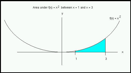
Using calculus, the exact size of this area is \(8 2/3\) or \(8.66\overline{6}\).

Discussion

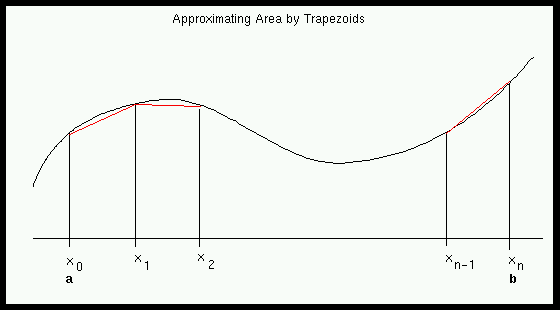
In what follows, we will not try to compute the desired area exactly. Rather, we will consider a fairly simple approach, called the trapezoidal rule, which can give good approximations of the area. In this approach, we break down a large area into small pieces and approximate each of the small pieces by a trapezoid (as shown below).

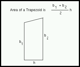
From geometry, we can compute the area of a trapezoid:

Then we can approximate the entire area under the curve by adding up the areas of the trapezoids.

More precisely, we first divide the interval \([a, b]\) into \(n\) equal pieces \(a=x_0, x_1, x_2, \dots, x_n=b\). Then we use the pieces to divide the overall areas into trapezoids. After we compute the area of each trapezoid, we add up these small areas. The final formula is:

where \(h = (b - a) / n\) and \(x_j = a + jh\) for \(j = 0, 1, 2, \dots, n\). This is the formula trapezoidal rule. (The interested reader should consult books in calculus or numerical methods for the details of this and other methods.)

To make this formula more concrete, we apply it to \(f(x) = x^2\) between \(x = 1\) and \(x = 3\) (as shown in an earlier figure), and we divide the interval \([1, 3]\) into five pieces. This gives: \(n = 5\); \(a = 1\); and \(b = 3\). The overall interval \([1, 3]\) has length \(2\); we divide it into five subintervals of length \(h = 2/5 = 0.4\). The \(x\) values are \(x_0 = 1\), \(x_1 = 1.4\), \(x_2 = 1.8\), \(x_3 = 2.2\), \(x_4 = 2.6\), and \(x_5 = 3\). The trapezoidal rule gives:

Theoretical Accuracy of the Trapezoidal Rule

While it is hard to predict the accuracy of approximations with the trapezoidal rule, we can make several useful observations.

• The trapezoidal rule relies upon the actual area under the graph being close to the area under the trapezoid.
• If the graph of the function is a straight line, then the trapezoids should give exact results. Otherwise the trapezoidal rule cannot be expected to be exactly correct.
• If we divide the interval \([a, b]\) into a large number of pieces, we can expect each trapezoid to be close to the actual area under the graph.
• As \(n\) gets bigger, the approximation of area using the trapezoidal rule should get better.

Practical Implications of Floating Point Error

Since floating-point numbers are not stored exactly, work with any individual floating-point number may involve a small amount of error. If these numbers are combined in many arithmetic operations, such small numerical errors sometimes can come together to significantly affect results.

Exercises

Driver: Student closer to the whiteboard

This part of the lab asks you to run and extend the provided trap-rule program, which computes area using the trapezoidal rule. You then will experiment with this program to investigate the effect of numerical errors. To get started run make trap-rule in your terminal to compile the provided code.

1. Review the trap-rule.c program and describe how it works. For example, how the table is produced? Why does the function area_l_to_r use the variable i? Why does the computation for xvalue give appropriate values for x values in the trapezoidal rule?

2. As noted above, the correct value of this area is \(8 2/3\) or \(8.66\overline{6}\) as determined with calculus. Write down how the computed approximations compare to this exact value as the number of intervals increases. To do this, run ./trap-rule.

3. The function area_l_to_r adds terms in the Trapezoidal Rule from first to last. For the function given, the terms get steadily larger as the function is increasing from left to right. A natural question arises regarding what might happen if the terms were added in the opposite order.

   Modify the program to include another function area_r_to_l, which adds the terms in the Trapezoidal Rule from last to first (i.e., from the \(n\)th term toward the initial term). Then, in the main loop, add another column to the table, for “Computing from R to L”.

   • Run the revised program, showing the results of both left-to-right and right-to-left computations.

   • Compare the results of the left-to-right and right-to-left computations. What patterns do you observe? What, if any, differences do you identify? Briefly explain what you see.