Trees

Summary

Trees are a class of data structures that organizes data in a hierarchical fashion. We explore trees briefly because they beautifully generalize the recursive definition of lists we have used extensively so far and as a functional language, Racket is particular adapt at handling this common form of data.

This reading was redeveloped for Fall 2020.

Lists as sequential structures

Recall that a list is defined recursively as a finite set of cases:

• The list is empty, or
• The list is non-empty and consists of a head element and the rest of the list, its tail.

In Scheme and Racket, you build lists with null (empty list) and cons (join a head and tail). You deconstruct lists with null? (check for empty list), car (grab the head), and cdr. Every other list operation we use can be built from those basics.

The structure of a list organizes its data in a sequential fashion. That is there is an ordering imposed by the list structure. For example, consider the following list of strings:

(define favorite-fruit '("pear" "apple" "peach" "grape" "olive"))

The recursive definition of a list implies that we will walk through the elements of the list in left-to-right order. For example, the following recursive function returns the first occurrence of a string that starts with the letter ‘p’:

(define find-first-p
  (lambda (l)
    (match l
      ['() (error "(find-first-p) not found!")]
      [(cons head tail)
       (if (string-prefix? head "p")
           head
           (find-first-p tail))])))

> (find-first-p favorite-fruit)
"pear"

Note that when used on our sample list, the function returns "pear" rather than "peach" because it encounters "pear" first.

We can use the sequential nature of lists to encode orderings, something that we will revisit at the end of the course when we talk about sorting algorithms. For now, we can observe that if assume that the list contains our favorite fruits in *decreasing order of favor, then we can easily define functions that retrieve our most favorite and least favorite fruits from the list:

(define most-favorite car)
(define least-favorite last)

> (most-favorite favorite-fruit)
"pear"
> (least-favorite favorite-fruit)
"olive"

(Note that most-favorite and least-favorite are directly defined to be the functions car and last, respectively, so they are themselves functions. In this sense, we can think of our definitions of most-favorite and least-favorite to be aliases or alternative names for car and last.)

In short, we can take advantage of the structure of a data type, here a list, to make defining operations easier as well as more efficient. This is the motivation behind the study of data structures which allow us to organize our data in various ways. Lists are our first example of such a data structure, and perhaps, the most fundamental in all of computing.

Not everything is naturally sequential

Lists work particular well when our data has a natural sequential interpretation or ordering to it. However, not all data behaves in this manner. For example, consider a management hierarchy that describes the groups that the managers of a company oversee:

• There are software developers that all report to the head of engineering.
• There are also testers that all report to the head of engineering.
• There are data analysts that report to the head of marketing.
• There are lawyers that report to the head of legal.
• The different group heads all report to the chief executive officer (CEO).
• The CEO reports directly to the board of directors.

The manner in which employees report to each other seems sequential in nature, but breaks down if we try to put them all into a list. We might try to do so with the board at the head of the list—since they’re the “top” of the management structure—and then work our way downwards.

'("Board"
  "CEO"
  "Head of Engineering"
  "Head of Marketing"
  "Head of Legal"
  "Software Developer"
  "Tester"
  "Data Analyst"
  "Lawyer")

The sequential nature of the list implies that the "CEO" reports to the "Board" which is correct. However, the "Head of Marketing" does not report to the "Head of Engineering"—they are actual equals in the management hierarchy! Likewise, a "Software Developer" doesn’t manage "Lawyers"; they do not have a direct relationship in terms of management.

Representing hierarchical structures with trees

It turns out that management hierarchies are not sequential in nature. They are, as suggested by their name, hierarchical. We can think of a hierarchy as imposing a parent-child structure on data. In this view, every child has one parent, but parents can have multiple children. In the above example, an example of a parent would be the "CEO" and its children would be the "Head of Engineering", "Head of Marketing" and "Head of Legal".

In computer programs, we represent hierarchies using a data structure called a tree. We might represent the management hierarchy above with a tree pictorially as follows:

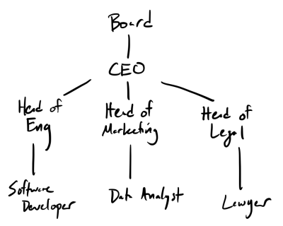
In the picture, a line between two names corresponds to a parent-child relationship where the parent is higher in the diagram than its child. We call each element of a tree a node of the tree. We also traditionally use tree terminology to describe the different parts of the structure:

• The "Board" is the root of the tree. It is the piece of data with no parent.
• "Software Developer", "Tester", "Data Analyst", and "Lawyer" are all considered leaves of the tree. Each of them have no children.
• Each of the heads have parents and children—we call them interior nodes of the tree. (Ok. That one isn’t really terminology from trees, but you get the point.)

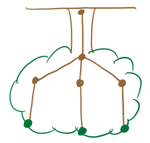
You might note that the "Board" is at the top of tree whereas the roots of the trees are found on the ground. That is correct! It turns out that the way computer scientists think of trees are upside-down:

A recursive interpretation of trees

Recall that the key insight behind performing recursive operations over lists was decomposing its structure in a way that we could identify a smaller sub-list inside of a larger list. We can do the same thing for trees. In our above example, the overall tree’s root is "Board", but note that this overall tree contains a smaller sub-tree: the sub-tree’s root is "CEO"! Furthermore, "CEO" contains 3 subtrees with each group head as roots.

With this in mind, we can define a tree recursively as follows. A tree is either:

• Empty, or
• Non-empty where it contains a datum and one or more children that are, themselves, trees. (We will sometimes use the term “subtrees” rather than “children”.)

Representing binary trees in Racket

In our example above, the maximum number of children any one of the nodes has is three: the "CEO" has three children. However, for the purposes of our first exploration into trees, we’ll first look at trees that have at most two children, so-called binary trees. When we work with binary trees, we refer to the first child as the “left child” or the “left subtree” and the second child as the “right child” or the right subtree.

How might we represent a tree using the Racket programming constructs we’ve seen so far? Note that the only difference between a list and a tree is that a list can only have one sublist whereas a binary tree can have up to two subtrees. This implies we can use all of our list constructs—null and cons for construction and car and cdr to decomposition. To represent multiple subtrees, we can use the pair construct we learned about previously: the “tail” of a tree will be a pair of subtrees instead of a single subtree!

Putting all of this together, we can represent a tree as follows:

• The empty tree is null.
• The non-empty tree (a node) is a list of three values, (v l r): v, the value at the node, l, the left subtree, and r, the right subtree.

Note that some perfer to represent the node as (cons v children) or (cons v (cons l r)), which saves a little space but at the cost of readability.

What do we do if a node has only one child? We use null for the first child. What do we do if a node has no children? (That is, if it’s a leaf?) We use null for both children.

For example, if we restrict our management hierarchy example to just its engineering and legal branches, we can represent this structure in Racket as follows:

(define management-tree
  (list "Board"
        null
        (list "CEO"
              (list "Head of Engineering"
                    null
                    (list "Software Developer"
                          null
                          null)
                    (list "Tester"
                          null
                          null))
              (list "Head of Legal"
                    null
                    (list "Lawyer"
                          null
                          null)))))

While we’ve structured the tree nicely, DrRacket is not so clear in printing it out.

> management-tree
'("Board"
  ()
  ("CEO"
   ("Head of Engineering" () ("Software Developer" () ()) ("Tester" () ()))
   ("Head of Legal" () ("Lawyer" () ()))))

Note that each node of the tree has the following skeleton:

(list <value> <subtree> <subtree>)

We always have three elements, even though there are sometimes one or zero subtrees. This keeps the structure of the tree uniform so we can operate it in the say way irrespective of the number of subtrees at each node.

Reading and writing tree definitions by hand is tedious and error prone. We should, therefore, write helper definitions to give better names to these definitions. Throughout, I recommend that you sketch out the design of each function from its description, if not outright implement it yourself. You can click on the buttons to look at the code we’ve written**, but we’d prefer you sketch your designs first.

binary-tree?

First, let’s write a predicate that tests whether a value is a binary tree. This predicate is a direct translation of the recursive definition of a tree into code. We can use the list and pair predicates from the standard library to directly capture our implementation strategy of encoding a tree as a list of three items, the first of which is a value and the remaining two of which are trees.

;;; (binary-tree? t) -> boolean?
;;;   t : any
;;; Returns true iff t is a binary tree.
(define binary-tree?
  (lambda (t)
    (or (empty-tree? t)                   ; the empty tree is a tree
        (and (pair? t)                    ; A list of exactly three elements
             (pair? (cdr t))
             (pair? (cddr t))
             (null? (cdddr t))
             (binary-tree? (cadr t))      ; Where element 1 is a tree
             (binary-tree? (caddr t)))))) ; And element 2 is a tree

empty-tree and empty-tree?

Next, let’s write some definitions to capture our notion of an empty tree, the base case of our recursive definition. We defined an empty tree to simply be null. So it is tempting to use null and null? as our empty tree value and test for whether we have an empty tree. However, even though a tree is really a list behind the scenes, we want to avoid thinking about these implementation details when writing tree code. Therefore, we’ll define empty-tree and empty-tree? to be aliases for null and null? which hides the fact that we implement trees as lists.

;;; empty-tree : tree?
;;; An alias for the empty binary tree.
(define empty-tree null)

;;; (empty-tree? t) -> boolean?
;;;   t : value
;;; Returns true iff is t is an empty binary tree.
(define empty-tree? null?)

Alternates for empty trees

Suppose we wanted to use a special value, such as 'empty or 'O or '_ for our empty trees. If we rely on empty-tree and empty-tree? in building our trees, we can easily make that change.

Consider how the definitions empty-tree and empty-tree? definitions above might change if we wanted to use '_ to represent the empty binary tree.

;;; empty-tree -> tree?
;;; An alias for the empty binary tree.
(define empty-tree '_)

;;; (empty-tree? t) -> boolean?
;;;   t : value
;;;
;;; Returns true iff is t is an empty binary tree.
(define empty-tree? 
  (lambda (t)
    (and (symbol? t) (eq? t '_))))

Creation

Now, we’ll write functions to create non-empty trees. (binary-tree value left right) creates a non-empty tree with the specified value and left and right sub-trees. Note that if a tree does not have either a left or right subtree, we can pass in the empty-tree for that respective argument. In addition to tree, we’ll also define a short-hand for the case where the tree has a value but no children, leaf.

;;; (binary-tree value left right) -> tree?
;;;   value : any
;;;   left : tree?
;;;   right : tree?
;;; Returns a non-empty tree with value at the root
;;; and the given left and right subtrees.
(define binary-tree list)

;;; (leaf value) -> tree?
;;;   value : any
;;; Returns a non-empty tree with no children (i.e., a leaf)
;;; with value at the root.
(define leaf
  (section binary-tree <> empty-tree empty-tree))

Tree Access

When given a non-empty tree, we would like to grab the individual components of that tree. There are three such components:

• The binary-tree-top this tree, i.e., and its root.
• The binary-tree-left this tree.
• The binary-tree-right this tree.

Keeping in mind the non-empty tree is really a pair of a value and a pair of subtrees, we can define these operations:

• (binary-tree-top t)
• (binary-tree-left t)
• (binary-tree-right t)

In terms of our pair projection functions car and cdr:

;;; (binary-tree-top t) -> any
;;;   t : tree?, (not (empty-tree? t))
;;; Returns the value at the root of this tree.
(define binary-tree-top car)

;;; (binary-tree-left t) -> any
;;;   t : tree?, (not (empty-tree? t))
;;; Returns the left child of this tree.
(define binary-tree-left cadr)

;;; (binary-tree-right t) -> any
;;;   t : tree?, (not (empty-tree? t))
;;; Returns the right child of this tree.
(define binary-tree-right caddr)

For example, we can use these tree projection functions to get at arbitrary parts of the tree:

> (binary-tree-top (binary-tree-right management-tree))
"CEO"
> (binary-tree-top 
   (binary-tree-left
    (binary-tree-right
     management-tree)))
"Head of Engineering"

Shorthands

You may note that when we regularly use lists, we start using procedures with short names, like caddr. Might we do the same for binary trees? Certainly. We’re designing the represention of binary trees and the associated procedures, we can do whatever we want. Let’s start with shorthands for the three main procedures. (All of these start with bt for binary-tree.)

(define btt binary-tree-top)
(define btl binary-tree-left)
(define btr binary-tree-right)

Think about how you might do a few more, such as the top of the left subtree, the top of the right subtree, or even the top of the left subtree of the right subtree, as in the example above.

> (bttlr management-tree)
"Head of Engineering"

(define bttl (o btt btl))
(define btll (o btl btl))
(define btrl (o btr btl))

(define bttr (o btt btr))
(define btlr (o btl btr))
(define btrr (o btr btr))

(define bttll (o bttl btl)) ; or (o btt btl btl)
(define btlll (o btll btl))
(define btrll (o btrl btl))

(define bttrl (o bttr btl))
(define btlrl (o btlr btl))
(define btrrl (o btrr btl))

(define bttlr (o bttl btr))
(define btllr (o btll btr))
(define btrlr (o btrl btr))

(define bttrr (o bttr btr))
(define btlrr (o btlr btr))
(define btrrr (o btrr btr))

Displaying trees

We can write a more elegant definition of our management tree using our tree creation functions:

(define management-tree
  (binary-tree
    "Board"
    empty-tree
    (binary-tree
      "CEO"
      (binary-tree
        "Head of Engineering"
        (leaf "Software Developer")
        (leaf "Tester"))
      (binary-tree
        "Head of Legal"
        empty-tree
        (leaf "Lawyer")))))

And our output is similarly unreadable.

'("Board"
  ()
  ("CEO"
   ("Head of Engineering" ("Software Developer" () ()) ("Tester" () ()))
   ("Head of Legal" () ("Lawyer" () ()))))

It doesn’t help much if we use the alternate form of empty trees.

'("Board"
  _
  ("CEO"
   ("Head of Engineering" ("Software Developer" _ _) ("Tester" _ _))
   ("Head of Legal" _ ("Lawyer" _ _))))

Rather than relying on Racket’s default output, let’s write a function, (display-binary-tree t), which displays the tree in a more digestible format. This function is inherently recursive:

• In the base case, we have an empty tree, so we display nothing.
• In the recursive case, we have a non-empty tree, so we display the current value and then recursively display the left-hand and right-hand trees.

We can translate this design directly into a recursive function.

(define display-binary-tree
   (lambda (tree)
     (when (not (empty-tree? tree))
       (display (btt tree))
       (newline)
       (display-binary-tree (btl tree))
       (display-binary-tree (btr tree)))))

However, we encounter a problem immediately: all the values are printed, one-per line, in a list!

> (display-binary-tree management-tree)
Board
CEO
Head of Engineering
Software Developer
Tester
Head of Legal
Lawyer

We need a way of visually distinguishing the different parent-child relations in this structure. One way to do this is to not print a linear list but a nested list using bullets. For example, this collection of bullets:

• Board
  • CEO
    • Head of Engineering
      • Software Developer
    • Head of Legal
      • Lawyer

This approach better represents the hierarchy visually. For example, it is clear that “Software Developer” is managed by the “Head of Engineering” and not the “CEO”.

How we implement this is a bit tricky! In addition to t, we need to introduce an additional parameter to our display function that remembers the current level of indentation we are at. This level goes up by 1 each time we recursively explore a child of the tree. We then use this value to print out an appropriate out of spaces per level.

We’ll explore recursive tree programming more in the next reading. For now, you can try designing and implementing this function, but don’t worry if it isn’t entirely clear how to proceed. We will discuss how to tackle recursive tree programming in the next reading!

;;; (display-binary-tree t) -> void?
;;;   t : tree?
;;; Prints tree t to the console in a well-formatted manner.
(define display-binary-tree
  (lambda (t)
    (let* (; The different levels of bullets
           [bullets (vector "* " "+ " "- " ". ")]
           ; The index of the last bullet
           [last-bullet (- (vector-length bullets) 1)]
           ; Choose the appropriate bullet for a level.
           [bullet
            (lambda (level)
              (vector-ref bullets (min level last-bullet)))])
      (letrec (; Display a binary tree at the appropriate indentation
               [helper
                (lambda (t indent)
                  (when (not (empty-tree? t))
                    (display (make-string (* indent 2) #\space))
                    (display (bullet indent))
                    (display (btt t))
                    (newline)
                    (helper (btl t) (+ indent 1))
                    (helper (btr t) (+ indent 1))))])
        (helper t 0)))))

Finally, let’s see how display-binary-tree works on our management-tree example:

> (display-binary-tree management-tree)
* Board
  + CEO
    - Head of Engineering
      . Software Developer
      . Tester
    - Head of Legal
      . Lawyer

Much nicer!

Conclusion

In this reading, we’ve introduced the recursive definition of a binary tree as well as associated functions for creating, manipulating, and displaying binary trees. You should study these implementations because they are excellent examples of advanced applications of lists and pairs!

Self Checks

Check 1: Another example of a tree (‡)

1. Come up with another example of a hierarchical structure that we could represent using trees. Describe the parent-child relationships in this example.
2. Use make-binary-tree and empty-tree to give a concrete example of your structure in Racket. Make sure your example involves a few levels so that you get practice writing our tree values. (You don’t have to write working code; just practice doing it. If you want working code, please copy and paste the procedures from above.)