Decomposition

Summary

We discuss one of the fundamental problem solving techniques in computing: algorithmic decomposition

As we learned in yesterday’s reading, an algorithm is a step-by-step procedure for solving a problem. These problems vary in scope from simple one-off tasks to complicated, generalized tasks that form the core of large, complex systems. For example, consider the problem of going through a web page and finding the links it contains. It turns out that a web page is plain text in a format known as hypertext markup language (HTML), so we can search the web page source file for occurrences of the text <a href="...">...</a> which correspond to links. For example, the beginning of this paragraph is rendered with the following HTML:

<p>As we learned in <a href="/csc151/readings/algorithm-building-blocks.html">yesterday’s reading</a>, an algorithm is a step-by-step procedure for solving a problem.
These problems vary in scope from simple one-off tasks to complicated, generalized tasks that form the core of large, complex systems.
For example, consider the problem of going through a web page and finding the links it contains.
It turns out that a web page is plain text in a format known as hypertext markup language (HTML), so we can search the web page source for for occurrences of the text <code class="language-drracket highlighter-rouge"><span class="nv">&lt;a</span> <span class="nv">href=</span><span class="s">"..."</span><span class="nv">&gt;&lt;/a&gt;</span></code> which correspond to links.
For example, the beginning of this paragraph is rendered with the following HTML:</p>

The paragraph contains one link corresponding to the text yesterday's reading. We will eventually learn how to do this in Racket, but even though we can’t write a program to do this yet, we can imagine that with proper library support that this is a simple task.

In contrast, the task of scraping web pages for links forms the basis of the algorithms that search engines use to rank webpages. For example, Google’s famous PageRank algorithm ranks the relevance of a webpage by the number of webpages that link to it. In order to do this, Google’s servers comb the Internet for webpages and scrapes their links, recording where they point to in a database.

PageRank itself is a complicated algorithm with many parts. However, what we should take away from this example is the fact that this complicated algorithm boils down to a simple task: scraping webpages for links. The process by which we take a complicated problem like ranking all webpages and distill it into a collection of smaller, easier-to-solve problems is called algorithmic decomposition.

Algorithmic decomposition is the lifeblood of a computer scientist. It is the primary skill that we employ to manage complexity in the problems that we solve. As such, we introduce this concept in this first week of the course to start getting you thinking with this mindset:

The problem that I am trying to solve can be decomposed into these smaller problems…

Visual Decomposition with Pictures

While we haven’t seen much of the Racket programming language yet, we know enough to introduce the basics of algorithmic decomposition with the images library introduced in yesterday’s reading. As a reminder, I encourage you not to read this passively; instead, enter the code interactively as you cover it in your reading. This will not only help you get used to typing out Racket code but also encourage you to play around and experiment with the language.

From last class period’s class, recall that we must include a require command in our definitions so that Racket knows we’re using the images library. We’ll also include the class library csc151 so that we have access to some additional functions that we will use.

#lang racket

(require 2htdp/image)
(require csc151)

After pressing Run, the interactions pane will now be ready for us to use functions from the image library.

Our initial reading on the Racket language introduce us to functions for drawing circles and rectangles:

> (circle 50 'outline "blue")

> (rectangle 75 50 'solid "red")

As well as functions that allow us to place images above and beside each other.

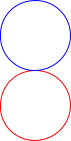
> (above (circle 35 'outline "blue")
         (circle 35 'outline "red"))

> (beside (rectangle 50 50 'solid "blue")
          (rectangle 50 50 'solid "red"))

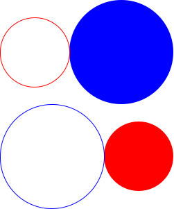
Let’s consider the problem of drawing the following more complex figure:

How might we approach this problem? We might start trying to cobble together random combinations of the functions we’ve seen so far, and we might stumble on a program that works. But such an approach—haphazardly trying stuff out until success is achieved—will not scale well when our problems get more complex!

Algorithmic decomposition is our primary problem solving strategy for systematically tackling complex problems. Rather than blundering into a solution, we proceed by:

1. Breaking up the original, complex problem into smaller, easier sub-problems to solve.
2. Solving each of those sub-problems in turn if they are easy enough to tackle directly, or further decomposing the sub-problems if they themselves are too complex!
3. Taking the solutions to each of those sub-problems and composing them together to form a solution to the original problem.

For example, we might decompose the problem of computing a student’s average assignment grade for a course as follows:

• Compute the sum of the student’s assignment grades (assuming they are all out of the same point total).
• Count the number of total assignments.
• Combine the two quantities via division to arrive at the final average.

We perform this process naturally in many situations, almost without thinking about it. However, when put into a novel situation, e.g., computer programming, you might neglect to go through these steps. It is therefore instructive to be explicit about your decomposition—luckily, this coincides with excellent programming practices, so your diligence is well-rewarded in this context.

Coming back to the proposed picture, let’s tackle the problem of drawing the image by breaking it down into smaller pieces. One way to do this is to analyze the image by row:

• The top row of shapes is a small, red circle outline followed by a large, blue filled-in circle.
• The bottom row of shapes is a large, blue circle outline followed by a small, red filled-in circle.
• The top and bottom rows are combined by stacking them on top of each other.

Now, when we go to write the code to produce this figure, we can translate this decomposition into code using the image library function and the define command to explicitly name each of the parts.

We can approach decomposition in either a bottom-up or top-down style of design. In a bottom-up style, we first implement the individual of pieces of the program and then we combine them to form the complete program. In a top-down style of design, we first partially implement the complete program and then implement the individual pieces. We’ll illustrate both styles of design below.

Bottom-up Design

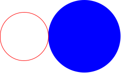
Let’s begin with the top row. We’ll define top-row to be the top row of circles using the circle and beside functions. Note that this define command should go into the definitions pane below your require command rather than in the interactions pane:

(define top-row
  (beside (circle 50 'outline "red")
          (circle 75 'solid "blue")))

After clicking Run to re-load these definitions, we can now go to the interactions pane and test our code. The practical effect of the define command is to make top-row an alias for the image, so we can simply type in top-row directly in the interactions pane to check our work:

> top-row

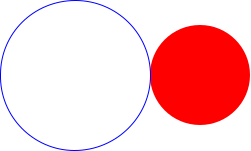
Next, we’ll define bottom-row to be the bottom row of circles in the definitions pane.

(define bottom-row
  (beside (circle 75 'outline "blue")
          (circle 50 'solid "red")))

And we’ll check our work in the interactions pane.

> bottom-row

Finally, let’s put it all together. As we discussed, the overall picture is obtained by stacking the top-row with the bottom-row which we can do with the above function:

(define circles
  (above top-row bottom-row))

We can check that circles is the image that we wanted in the interactions pane. (Remember to re-Run your program in DrRacket so that circles has been defined!)

> circles

Top-Down Design

With top-down design, rather than starting with top-row and bottom-row, we start with the overall program circles. We have identified that circles is a stack of two rows of images, so we know that the definition of circles will involve above. However, we have not defined top-row and bottom-row yet—what do we fill in for the arguments to above?

The csc151 library defines a special value {??} which represents a hole in our program yet-to-be filled in. {??} acts as a syntactically valid placeholder, reminding us that we should replace {??} with an eventual implementation.

; Note: if you are following live, remove circles, top-row, and
;       bottom-row from your source so you can try this out!
(define circles
  (above {??} {??}))

When run, our code produces the following error:

Hole encountered!  Fill me in!

And highlights the hole that it encountered in DrRacket, indicating that we still have work to do! Of course, we know the work that must be done already—we need to implement each row. Let’s do that for top-row first.

(define top-row
  {??})

Note that we can use our hole value as a placeholder to be able to write out the syntax of a define correctly and ensure that we get it right. Of course, when we run this code, we the Hole encountered! Fill me in! error, but we at least know that we have all the keywords and parentheses in the right place.

Once we define top-row as before:

  (beside (circle 50 'outline "red")
          (circle 75 'solid "blue")))

We can now fill in the corresponding hole in circles:

(define circles
  (above top-row {??}))

Finally, we can define bottom-row just like before and then complete the definition of circles:

(define circles
  (above top-row bottom-row))

Top-down vs. Bottom-up Design

You might wonder which sort of design—top-down or bottom-up—to use when writing your programs. The short answer is that it depends on the kind of problem you are tackling and your own personal preference. Sometimes you might see how to immediately implement the smaller pieces of a program in which you can start with those pieces and then build up to the overall program. In other cases, you might not see the pieces and want to essentially outline how the program ought to behave in code, similar to the bulleted list we identified for the design of shapes. In this case, you can use top-down design to write this outline and then fill it in incrementally. Either strategy is valid—be willing to experiment early on with both styles to discover your preferences and be flexible in how you design your code!

Decomposition In Code

Finally, let’s look at the big picture. Take a look at the complete program that we wrote in the definitions pane:

#lang racket

(require csc151)
(require 2htdp/image)

(define top-row
  (beside (circle 50 'outline "red")
          (circle 75 'solid "blue")))

(define bottom-row
  (beside (circle 75 'outline "blue")
          (circle 50 'solid "red")))

(define circles
  (above top-row bottom-row))

Note how our decomposition strategy has been enshrined in the code. That is, our approach to solving the problem of drawing the grid of circles is evident in the code:

circles is defined to be a stack of a top-row and bottom-row. Each of the rows contain two circles of varying color, shape, and sizes.

By employing algorithmic decomposition in our problem solving and programming, we not only gain the able to make tangible progress in solving the problem; our code is much more readable as a result! As we move forward in the course, always approach problems with decomposition in mind even if they are easy to solve at first. Honing this skill early on in your programming journey will prepare you well for the complex problems will encounter later in the semester!

Self Checks

Check 1: Readability (‡)

Here is an alternative version of the code to produce the image of this reading.

#lang racket

(require 2htdp/image)

(define circles
  (above (beside (circle 50 'outline "red")
                 (circle 75 'solid "blue"))
         (beside (circle 75 'outline "blue")
                 (circle 50 'solid "red"))))

Paste this code into a fresh DrRacket tab’s definitions pane and verify that circles produces the same image as before.

Compare and contrast the final version of the code the reading with this version. Answer each of the following questions in a few sentences each.

• Which version is more concise? Why?
• Which version do you find more understandable? Why?
• Which version allows you to better predict the results without running the program? Why?

Check 2: Alternative Decomposition (‡)

There are many ways to decompose a problem, many of which are equivalent, but many produce subtlety different solutions. The decomposition we chose in the reading was one where we recognized the image was two rows stacked on top of each other. Try writing the code corresponding to a decomposition where we think of the image as two columns placed side-by-side. Does this result in an identical image? Why or why not?